[1]:

from eddy import rotationmap
import numpy as np

5 - Self-Gravity and Pressure Supported Disks¶

It is becoming ever apparent that the background motion in a disk is subtly perturbed away from a pure Keplerian profile of $v_{\phi} \propto r^{-0.5}$ due to either the background pressure support slowing the rotation (e.g., Dullemond et al., 2020) or the self-gravity of the disk hastening the rotation (e.g., Veronesi et al., 2021). If the goal of your science is to better understand these properties then undertaking a full modeling of the $v_{\phi}$ profile is the best idea. However, if your goal is just to remove some average background profile to search for localized deviations then parameterization adopted in eddy might be worth a shot.

Parameterization¶

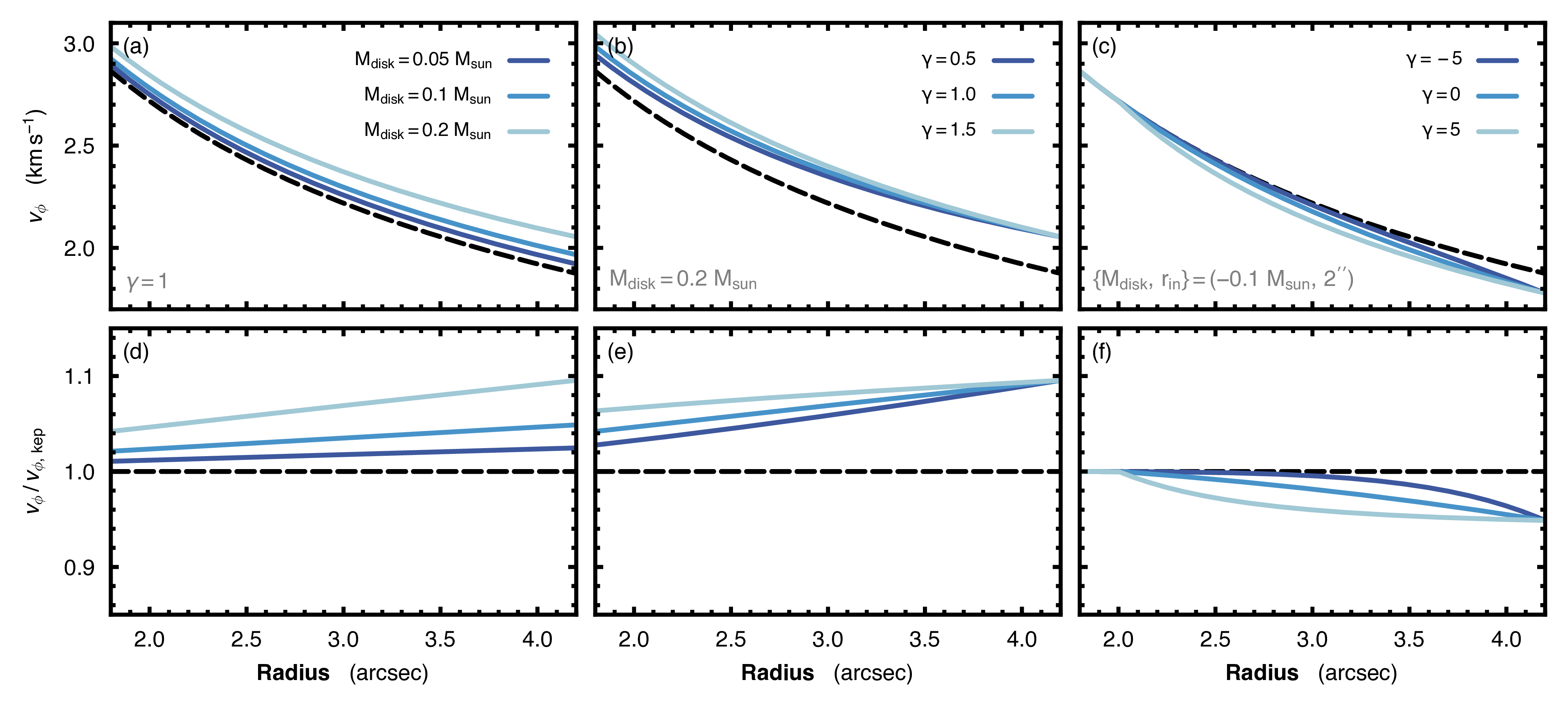
For a 2D, purely Keplerian disk the rotation profile is given by

$v_{\phi} = \sqrt{\frac{GM_*}{r}},$

where $M_*$ is the dynamical mass of the central star. This can be modified to include an additional radial-dependent mass component, $M_d(r)$ , that describe the disk mass within cylindrical radius $r$ (we explain why we have adopted this simplification later on). This gives a modified rotation curve of

$v_{\phi} = \sqrt{\frac{G(M_* + M_d(r))}{r}}.$

Assuming a power-law surface density profile of the form, $\Sigma(r) = \Sigma_0 \times r^{-\gamma}$ , then $M_d(r)$ is given by

$M_d(r) = M_{\rm disk} \times \frac{r^{2 - \gamma} - r_{\rm in}^{2 - \gamma}}{r_{\rm out}^{2 - \gamma} - r_{\rm in}^{2 - \gamma}},$

with $r_{\rm in}$ and $r_{\rm out}$ describing the disk inner and outer edge, respectively, and $M_{\rm disk}$ is the total disk mass. Note that for the commonly assumed $\gamma = 1$ case this is a simple linear interpolation between $r_{\rm in}$ and $r_{\rm out}$ .

These parameters can be controlled with the parameter names 'mdisk', 'gamma', 'r_in' and 'r_out' (note here to differentiate these from the 'r_min' and 'r_max' parameter that describe the mask).

Although the parameterization described above was motivated by the need for a hastening of the disk’s rotation due to the added gravitational potential of the disk, this functional form allows for a handy form to also account for the pressure support in the outer edge of the disk. This connection can most easily be seen when you consider the slowing of the disk as due to a radially dependent negative disk mass.

With this interpretation you can broadly relate the parameters to properties of the pressure support:

'mdisk' - Sets the magnitude of sub-Keplerian rotation.
'r_in' - Sets the radius where the rotation profile deviates from Keplerian rotation, likely the start of the exponential tail in the surface density profile.
'r_out’ - Sets the radius beyond which the rotation curve looks Keplerian again, but around a star with a reduced dynamical mass.
'gamma' - Sets how quickly the velocity profile transforms between 'r_in' and 'r_out'.

This figure from Teague et al. (2022) shows how these parameters can be used to mimic a super-Keplerian (panels a, b, d and e) and sub-Keplerian (panels c and f) rotation curve where the black dashed line shows a purely Keplerian profile.

c2a769c6a8c54d21839b25e5948ddbb3

Application to a Self Gravitating Disk¶

[2]:

# coming soon

Application to a Pressure Supported Disk¶

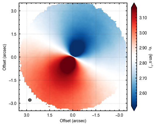
First we load up the data from Teague et al. (2022). The v0 and dv0 maps can be obtained from eddy Dataverse, or using the cell below.

[3]:

import os
if not os.path.exists('TWHya_CO_32_cube_gtv0.fits'):
    !wget -O TWHya_CO_32_cube_gtv0.fits -q https://dataverse.harvard.edu/api/access/datafile/7070646
if not os.path.exists('TWHya_CO_32_cube_dgtv0.fits'):
    !wget -O TWHya_CO_32_cube_dgtv0.fits -q https://dataverse.harvard.edu/api/access/datafile/7070645

Note here we’re using the downsample parameter to speed things up and setting a field of view of 7 arcseconds with the FOV argument.

[4]:

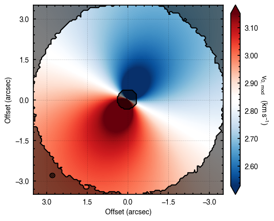
cube = rotationmap('TWHya_CO_32_cube_gtv0.fits', FOV=7.0, downsample=2)
cube.plot_data()

Assuming uncertainties in TWHya_CO_32_cube_dgtv0.fits.

To start we try and fit a simple Keplerian model. Remember to mask out those inner regions where beam smearing becomes an issue.

[5]:

# Dictionary to contain the disk parameters.

params = {}

# Start with the free variables in p0.

params['x0'] = 0
params['y0'] = 1
params['PA'] = 2
params['mstar'] = 3
params['vlsr'] = 4

# Provide starting guesses for these values.

p0 = [0.0, 0.0, 151., 0.81, 2.8e3]

# Fix the other parameters.

params['inc'] = 5.8
params['dist'] = 60.1
params['r_min'] = 2.0 * cube.bmaj

# Run the sampler.

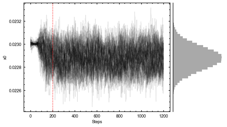
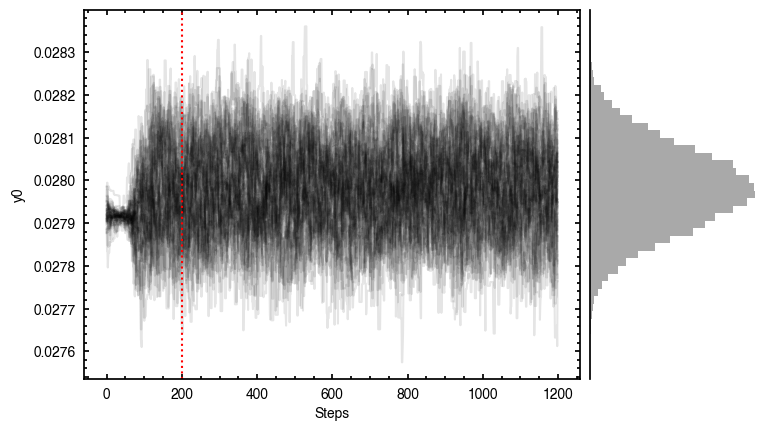
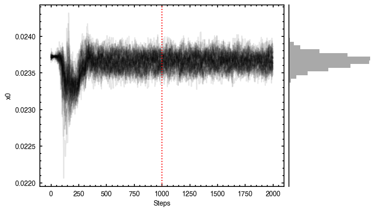
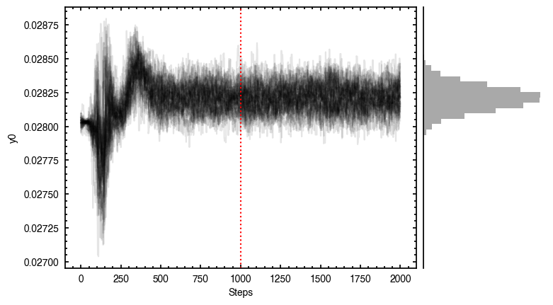
samples = cube.fit_map(p0=p0, params=params, nwalkers=64, nburnin=200, nsteps=1000)

Assuming:
        p0 = [x0, y0, PA, mstar, vlsr].
Optimized starting positions:
        p0 = ['2.30e-02', '2.79e-02', '1.52e+02', '7.75e-01', '2.84e+03']

100%|███████████████████████████████████████| 1200/1200 [01:10<00:00, 17.10it/s]

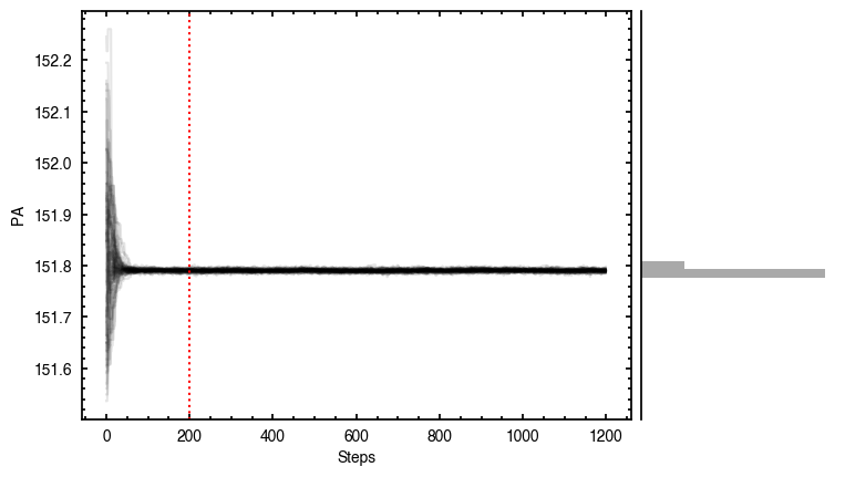
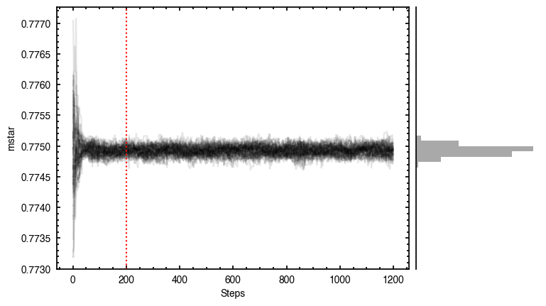
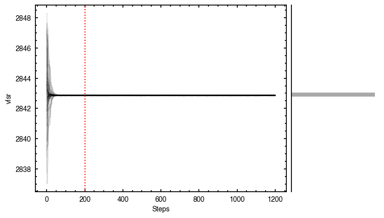
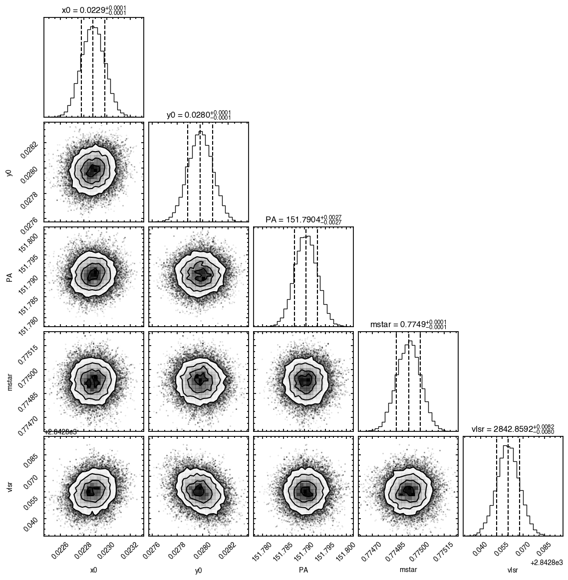
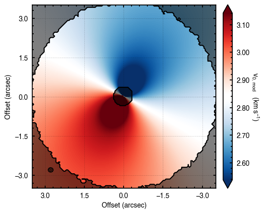
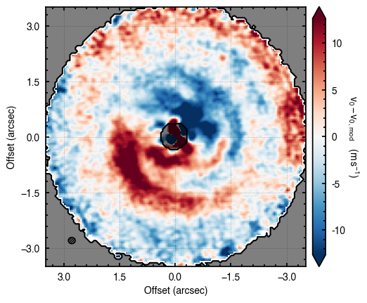
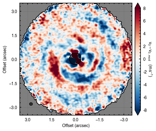
Although we get nice convergence of the walkers with seemingly independent posterior distributions, the residuals highlight that there’s clearly some residual structure. Once major component is the large spiral arm which is discussed in the aforementioned paper. However, there’s a clear red / blue residual along the major axis that can be attributed to sub-Keplerian rotation (see Fig. 5 in the Appendix of Teague et al. 2019a).

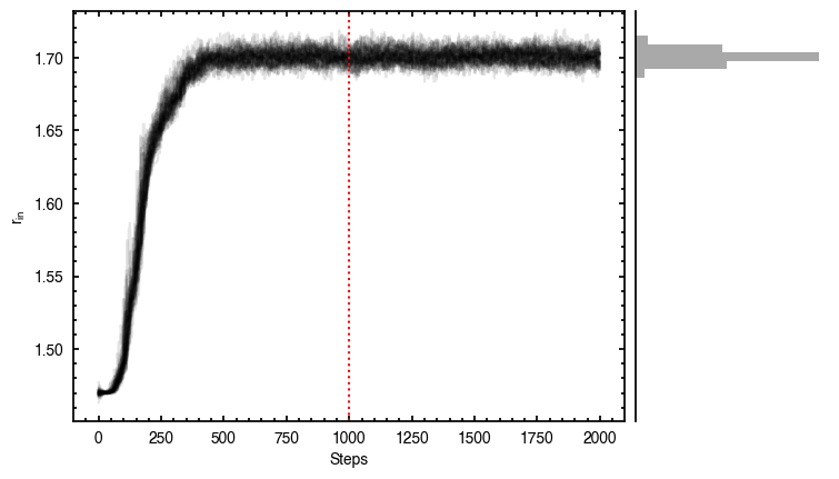
To account for this structure we can use the parameterization described above. Here we set 'r_out' to the disk outer edge, 4 arcseconds, as this should be the slowest part of the rotation.

[6]:

# Dictionary to contain the disk parameters.

params = {}

# Start with the free variables in p0.

params['x0'] = 0
params['y0'] = 1
params['PA'] = 2
params['mstar'] = 3
params['vlsr'] = 4
params['r_in'] = 5
params['gamma'] = 6
params['mdisk'] = 7

# Provide starting guesses for these values.

p0 = [0.0, 0.0, 151., 0.81, 2.8e3, 1.0, 1.0, 0.0]

# Fix the other parameters.

params['inc'] = 5.8
params['dist'] = 60.1
params['r_min'] = 2.0 * cube.bmaj
params['r_out'] = 4.0

# Run the sampler.

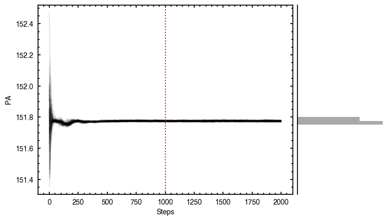
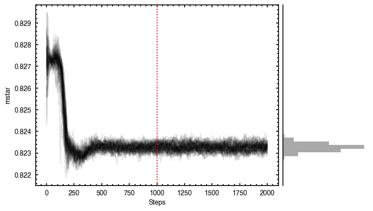
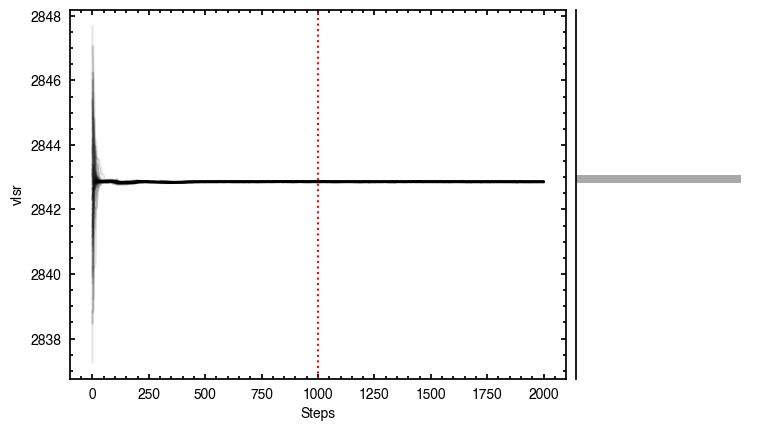
samples = cube.fit_map(p0=p0, params=params, nwalkers=64, nburnin=1000, nsteps=1000)

Assuming:
        p0 = [x0, y0, PA, mstar, vlsr, r_in, gamma, mdisk].
Optimized starting positions:
        p0 = ['2.37e-02', '2.80e-02', '1.52e+02', '8.27e-01', '2.84e+03', '1.47e+00', '9.19e-01', '-1.37e-01']

100%|███████████████████████████████████████| 2000/2000 [02:22<00:00, 13.99it/s]

../_images/tutorials_tutorial_5_10_2.png

../_images/tutorials_tutorial_5_10_3.png

../_images/tutorials_tutorial_5_10_4.png

../_images/tutorials_tutorial_5_10_5.png

../_images/tutorials_tutorial_5_10_6.png

../_images/tutorials_tutorial_5_10_7.png

../_images/tutorials_tutorial_5_10_8.png

../_images/tutorials_tutorial_5_10_9.png

../_images/tutorials_tutorial_5_10_10.png

../_images/tutorials_tutorial_5_10_11.png

../_images/tutorials_tutorial_5_10_12.png

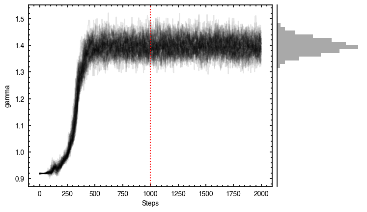
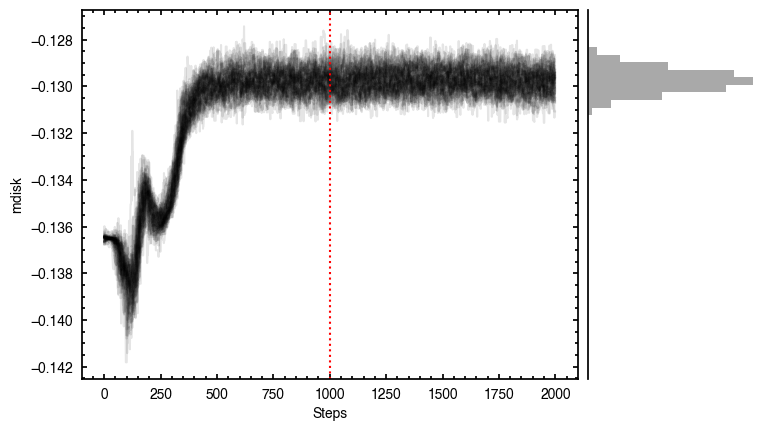
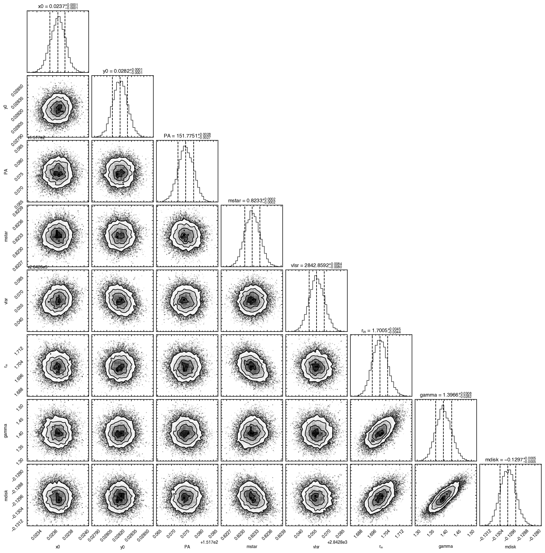
Clearly this does a much better job of removing those outer residuals and leaving a more prominent spiral pattern.