1 - Fitting Rotation Maps¶

A common task for analyses of protoplanetary disks is to infer their geometrical properties, namely the source centre, $(x_0,\, y_0)$ , the inclination $i$ , position angle, ${\rm PA}$ , and stellar (dynamical) mass, $M_{\rm star}$ , by fitting a simple Keplerian rotation pattern to a measured rotation pattern. In this notebook we’ll look at how to use eddy to fit rotation maps, provide some constraints on these model parameters and search for structure in the residuals.

TW Hya - A Geometrically Thin Case¶

Getting the Data¶

In this tutorial, we’ll use $^{12}{\rm CO} \,\, (2-1)$ observations of TW Hya, described in Huang et al. (2018), and is available for download here.

[1]:

import os
if not os.path.exists('TWHya_CO_cube.fits'):
    !wget -O TWHya_CO_cube.fits -q https://dataverse.harvard.edu/api/access/datafile/:persistentId?persistentId=doi:10.7910/DVN/PXDKBC/QULHRK

Making a Rotation Map¶

The first thing we need is a rotation map, i.e. a map of the line-of-sight velocity for each pixel. There’s a few different ways to make this from your data, for example a traditional intensity-weighted average velocity (first moment map), which is what CASA produces with its immoments command, or ‘quadratic’ method as advocated for in Teague & Foreman-Mackey (2018) and implemented in bettermoments, or analytical fits, such as in GMoments. Each of these methods have their benefits, and you should consider which is the most appropriate statistic for the scienece you want to do.

As we are performing model fitting, we also want some idea of the uncertainties on the line-of-sight velocities. Unfortunately, CASA does not calculate these for you, but bettermoments does, following the uncertainties described in Teague (2019). These aren’t essential for use with eddy as you are able to assume the uncertainties are some fraction of the line-of-sight velocity - not ideal, but it usually works.

This cell below will use bettermoments to create a rotation map using the quadratic method, masking all points which are $<5\sigma$ .

[ ]:

!bettermoments TWHya_CO_cube.fits -clip 5

Downloading the Rotation Map¶

If you do not want to make your own line-of-sight velocity maps, you can download ones already made with bettermoments through the eddy Dataverse. This will contain the line-of-sight velocity map, TWHya_CO_cube_v0.fits and the associated uncertainty, TWHya_CO_cube_dv0.fits. If you have gone through the steps above you’ll be ready, otherwise we can grab the necessary files from Dataverse.

[1]:

import os
if not os.path.exists('TWHya_CO_cube_v0.fits'):
    !wget -O TWHya_CO_cube_v0.fits -q https://dataverse.harvard.edu/api/access/datafile/:persistentId?persistentId=doi:10.7910/DVN/KXELJL/VPLAM7
if not os.path.exists('TWHya_CO_cube_dv0.fits'):
    !wget -O TWHya_CO_cube_dv0.fits -q https://dataverse.harvard.edu/api/access/datafile/:persistentId?persistentId=doi:10.7910/DVN/KXELJL/BLMBH0

Loading up the Data¶

Within eddy we have defined a rotationmap class which provides all the functionality we’ll need. Let’s load it up along with other standard imports.

[1]:

import matplotlib.pyplot as plt
from eddy import rotationmap
import numpy as np

In addition to the path to the data cube we want to fit, there are three extra arguments we need.

Uncertainties¶

If you have a map of the uncertainties for each pixel, they can be included with the uncertainty argument. If you don’t, that’s OK as it was assume a 10% uncertainty on each pixel by default. The uncertainty can be changed on the fly through the cube.error parameter. Note that this is actually a pretty bad approximation so it is highly recommend to include proper uncertainties. If you use the bettermoments naming convention, you can skip the uncertainty argument as it will search for the file *_dv0.fits in the same directory.

Downsampling¶

We have also downsampled the data so that we only included (roughly) spatially independent pixels. Additionally you can enter any integer to downsample by that factor. This is optional but useful for speeding up things when you’re playing around.

Field of View¶

Using the FOV argument we have also clipped the cube down to the region of interest. Be aware, when eddy is making a rotation map, it makes it for the full image, even if you’re only fitting an inner region defined by a mask. Clipping down to the region of interest (masked region) will considerably speed up the process.

[2]:

cube = rotationmap(path='TWHya_CO_cube_v0.fits',
                   uncertainty='TWHya_CO_cube_dv0.fits',
                   downsample='beam',
                   FOV=7.0)

Data Inspection¶

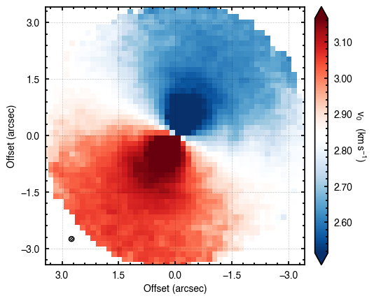
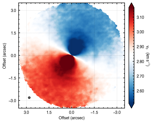
We can also inspect the data to make sure it looks how we’d expect it to. All we’re looking for here is that the downsampling and field of view that were chosen look reasonable, and you can see the typical dipolar morphology indicative of a rotating source.

[3]:

cube.plot_data()

../_images/tutorials_tutorial_1_11_0.png

There are a few other tools that may be useful for a quick inspection of the data described in TBD.

Fitting the Rotation Map¶

Here we describe how to fit the data using the fit_map function. For this introductory case, we assume a geometrically thin, Keplerian disk model where

$v_0 = \sqrt{\frac{GM_{\rm star}}{r}} \cdot \cos \phi \cdot \sin i + v_{\rm LSR} \quad \text{or} \quad v_0 = v_{\rm kep} \cdot \cos \phi \cdot \sin i + v_{\rm LSR}$

where $r$ is the cylindrical distance from the star (converted from angular distances in arcseconds to au by multiplying by the source distance, $d$ ), $\phi$ is the polar angle of the pixel (measured east of north relative to the redshifted major axis) and $v_{\rm LSR}$ is the systemic velocity.

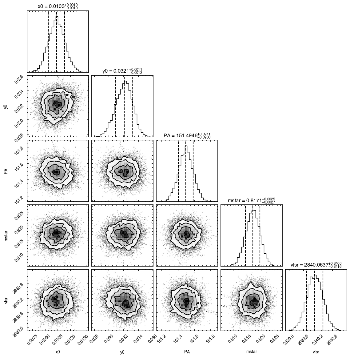
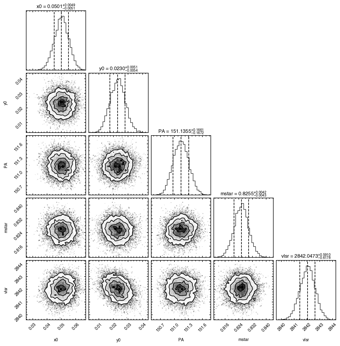
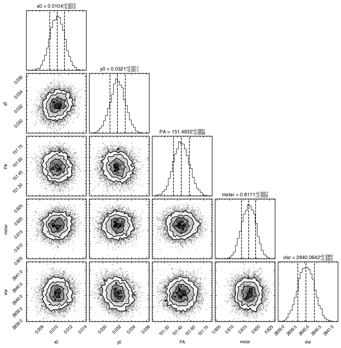
For the fitting, we need to know which of these values we’re fixing and which we want to fit for. Given the extreme degeneracy between $i$ and $M_{\rm star}$ for low inclination disks, a good idea is to either fix $i$ to a value found from fitting the continuum, or adopt a literature value for the dynamical mass. For this example we want to find the source center, $(x0,\, y0)$ , the position angle of the disk, ${\rm PA}$ , the stellar mass $M_{\rm star}$ and the systemic velocity, $v_{\rm LSR}$ , while holding the inclination fixed at $i = 5.8^{\circ}$ , the value adopted in Teague et al. (2019).

Thus we have our free model parameters, $\Theta = \{x_0,\, y_0,\, {\rm PA},\, M_{\rm star},\,v_{\rm LSR}\}$ , and our fixed model parameters, $\Theta_{\rm fixed} = \{i,\, d\}$ .

We the provide two things to fit_map:

p0: a list of the initial guesses for the free parameters, $\Theta$ .
params: a dictionary containing both the indices of the free variables in p0 as an integer and the fixed values for all other variables as a float.

With this dictionary framework it is possible to hold certain parameters fixed and others free. In particular, if you know the rotation direction of the disk (controlled by the sign of $i$ , discussed in a later tutorial) then this is a good parameter to fix.

[4]:

# Dictionary to contain the disk parameters.

params = {}

# Start with the free variables in p0.

params['x0'] = 0
params['y0'] = 1
params['PA'] = 2
params['mstar'] = 3
params['vlsr'] = 4

# Provide starting guesses for these values.

p0 = [0.0, 0.0, 151., 0.81, 2.8e3]

# Fix the other parameters. All values which are to be fixed must be floats.

params['inc'] = 5.8    # degrees
params['dist'] = 60.1   # parsec

The fit_map function has several steps:

Using the initial values in p0 to deproject the data, it will create a mask of the regions to fit. Note that if the initial guesses are poor, the mask will not be well defined. This can be circumvented with the niter argument, discussed later.
If optimize=True, which is strongly recommended, it tries to find the values in p0 which maximize the likelihood function. Using these updated p0 values it will then recalculate the regions to fit.
It will the make any specified diagnostic plots.
It will return any requested products.

[5]:

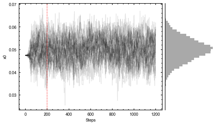
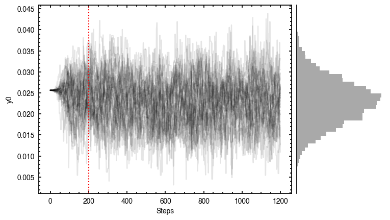
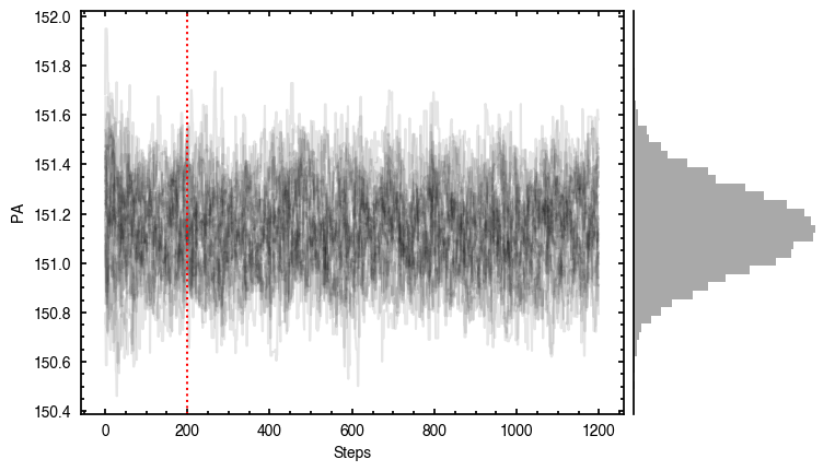
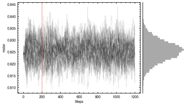
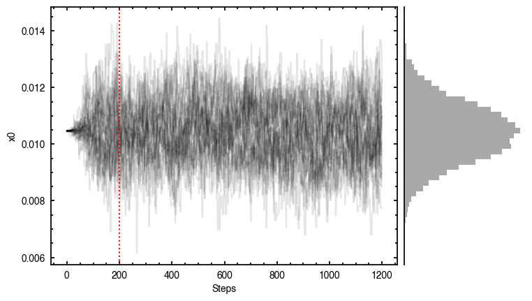
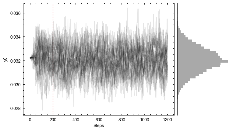
samples = cube.fit_map(p0=p0, params=params,
                       nwalkers=32, nburnin=200, nsteps=1000)

Assuming:
        p0 = [x0, y0, PA, mstar, vlsr].
Optimized starting positions:
        p0 = ['1.05e-02', '3.22e-02', '1.51e+02', '8.17e-01', '2.84e+03']

100%|██████████████████████████████████████| 1200/1200 [00:06<00:00, 187.49it/s]

../_images/tutorials_tutorial_1_15_2.png

../_images/tutorials_tutorial_1_15_3.png

../_images/tutorials_tutorial_1_15_4.png

../_images/tutorials_tutorial_1_15_5.png

../_images/tutorials_tutorial_1_15_6.png

../_images/tutorials_tutorial_1_15_7.png

../_images/tutorials_tutorial_1_15_8.png

../_images/tutorials_tutorial_1_15_9.png

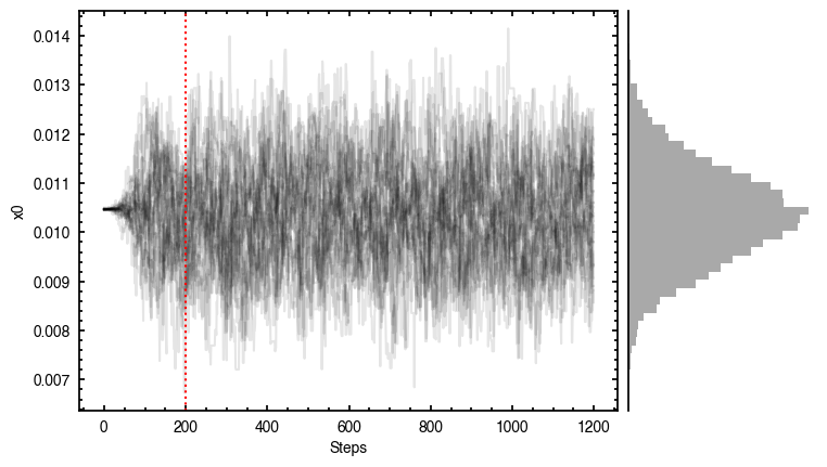
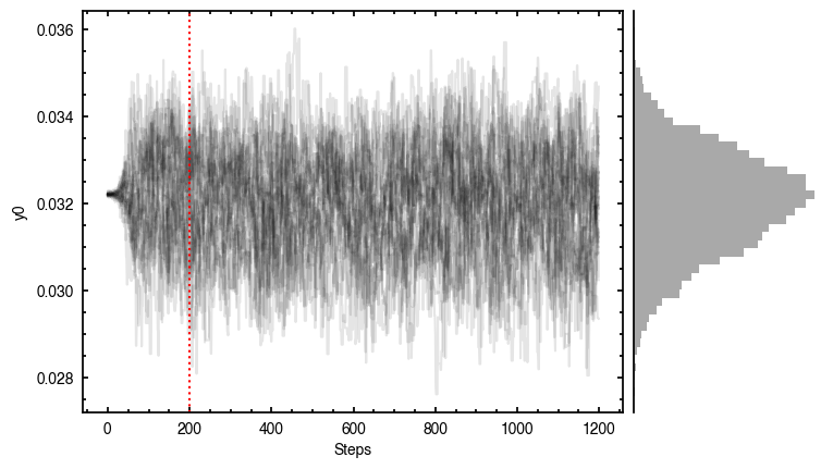
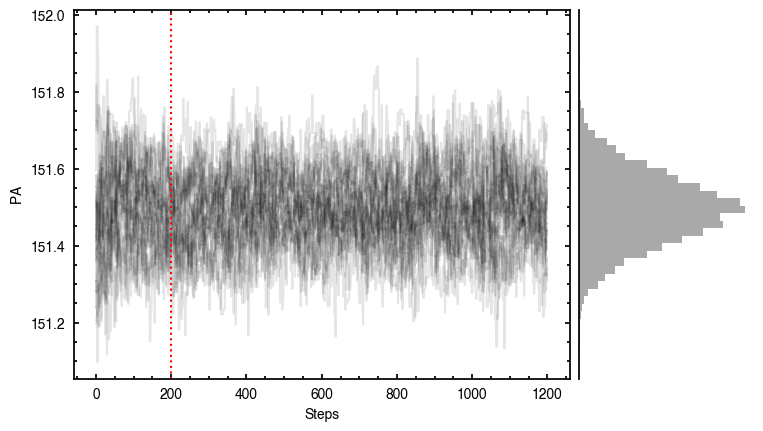
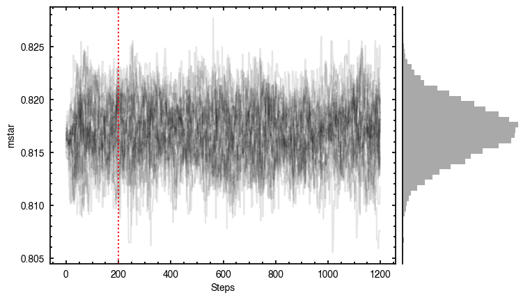
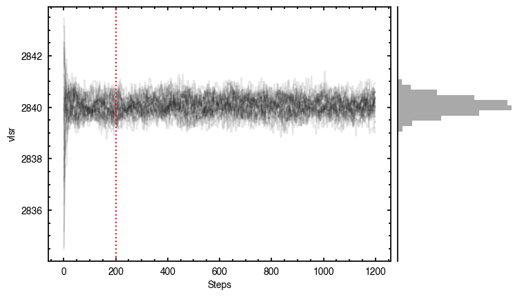
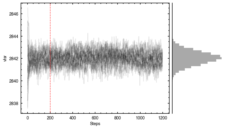
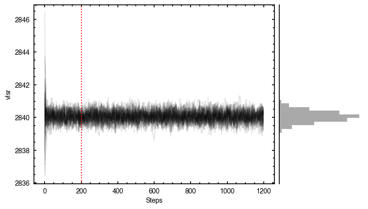
Note that through these tutorials, we use only a small number of steps for the MCMC as we just want to demonstrate the functionality of eddy. When using this for publishable results, it is strongly recommended to perform checks on the walkers to make sure they have sufficiently burnt in and are converged.

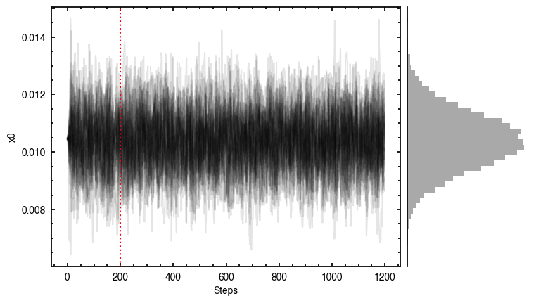
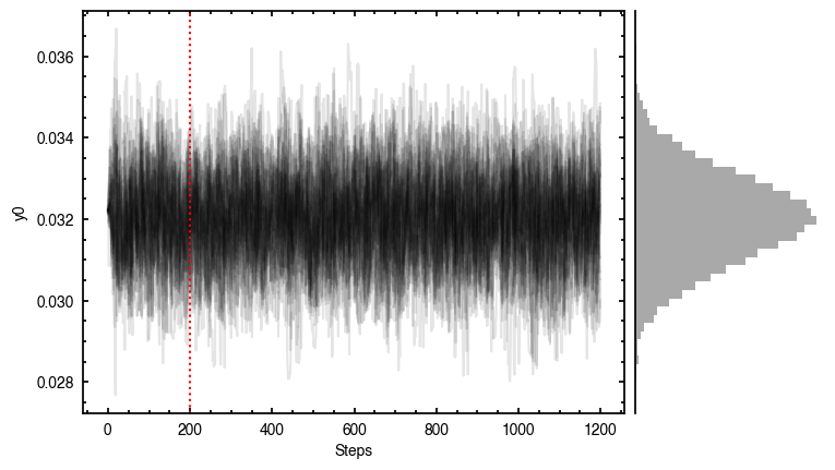
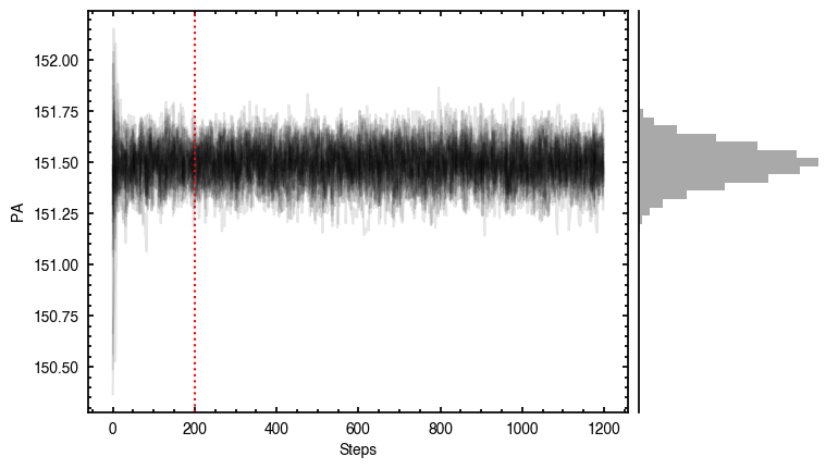
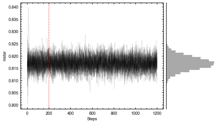
Diagnostic Plots¶

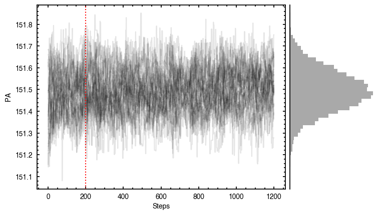
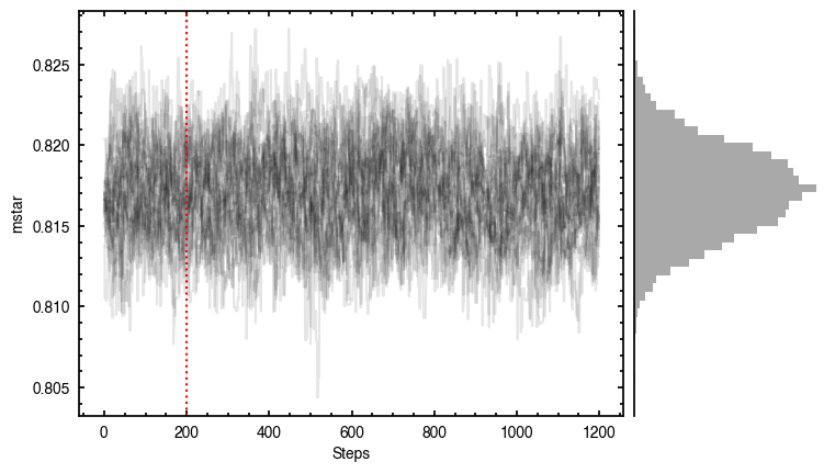
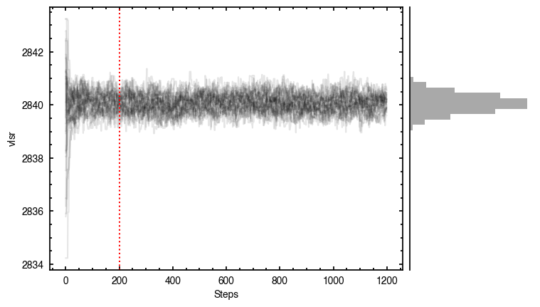
By default, fit_map will produce all the diagnostic plots. You can select which plots you want using the plots argument, which takes either a single (string) value, or a list of strings. The available options are:

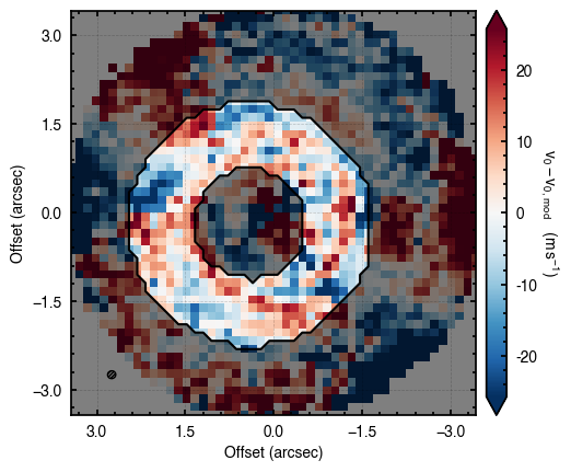
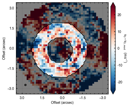
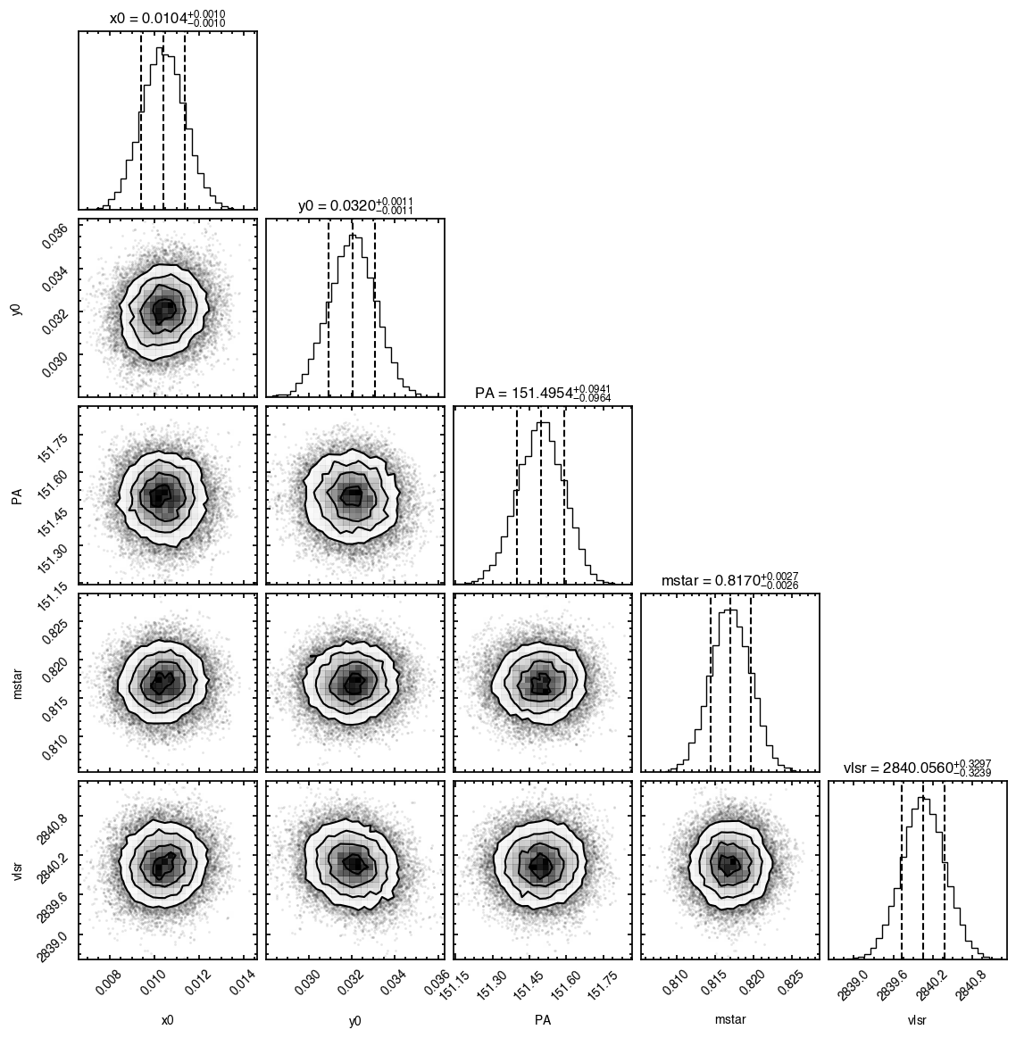
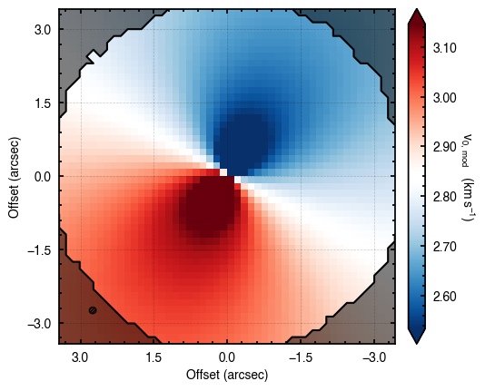
'walkers' - Shows the traces of the walkers for each parameter. In each panel, the dashed red line shows the end of the burn-in period. The histogram shows the collapsed posterior distribution for all samples taken after the burn-in period.
'corner' - A typical corner (covariance) plot using corner.py from Dan Foreman-Mackey. The labels will show the median value with uncertainties representing the 16th to 84th percentile range.
'bestfit' - A plot of the best-fit model (using the median value of the posteriors) with the mask overlaid.
'residual' - A plot of the residuals between the data and the best fit model with the mask overlaid.

For example, if you wanted to just plot the residual you would use, plots='residual', while for plots of the walkers and the corner plot you would use plots=['walkers', 'corner']. If you would like no plots, you can use plots='none' (careful to use a string here as plots=None is interpreted as the default of all plots).

Returned Products¶

There are several different statistics or data products that can be returned after the MCMC, controlled with the returns argument. As for the plots, this takes either a single string or a list of strings. The available options are:

'samples' - A (nsteps, nparams) shaped array of the posterior samples after the burn-in period. This has not been thinned, so must be done by hand if necessary.
'percentiles' - A (3, nparams) shaped array of the 16th, 50th and 84th percentiles of each parameter’s posterior distribution, a proxy of the standard deviation for a Gaussian distribution.
'lnprob' - A nsteps sized array of the log-probability for each posteroir sample.
'model' - A 2D array of the best-fit model using the median value from the samples.
'residuals' - A 2D array of the residuals after subtracting the best-fit model from the data.
'dict' - A params dictionary where the free parameters have been replaced with the median values of the posterior distributions.

By default eddy will just return the samples from the MCMC.

Masking Data¶

Oftentimes it is useful to only fit a specific region of your rotation map, perhaps because you are only interested in a spatial radial region. Within eddy, you can define a map based on the disk-frame $(r,\, \phi)$ coordinates and / or on the value of $v_0$ to avoid cloud-contaminated velocities.

For each of these optionn, r, phi and v, you can specify the minimum and maximum value to include or exclude in your mask. For example, to only include the regions between $0.5^{\prime\prime}$ and $1.0^{\prime\prime}$ we would use,

params['r_min'] = 0.5
params['r_max'] = 1.0

If instead we wanted to fit everywhere except a radial region between $0.5^{\prime\prime}$ and $1.0^{\prime\prime}$ and an azimuthal region where $|\phi| \leq 30^{\circ}$ we would use,

params['r_min'] = 1.0
params['r_max'] = 2.0
params['exclude_r'] = True
params['phi_min'] = -30.0
params['phi_max'] = 30.0
params['exclude_phi'] = True

In addition, there is the key 'abs_phi' which will assume $\phi$ is mirrored about the major axis of the disk to aid in defining regions on either side of the minor axis, for example. Note that, as mentioned before, the mask generation will adopt the initial geometrical properties provided to the fit_map function. If these are wildly off the true values, the resulting mask will not be very good.

[6]:

# fit only an annulus of points

params['r_min'] = 1.0
params['r_max'] = 2.0

samples = cube.fit_map(p0=p0, params=params,
                       nwalkers=32, nburnin=200, nsteps=1000,
                       plots=None)

Assuming:
        p0 = [x0, y0, PA, mstar, vlsr].
Optimized starting positions:
        p0 = ['4.75e-02', '2.56e-02', '1.51e+02', '8.24e-01', '2.84e+03']

100%|██████████████████████████████████████| 1200/1200 [00:06<00:00, 187.79it/s]

../_images/tutorials_tutorial_1_23_2.png

../_images/tutorials_tutorial_1_23_3.png

../_images/tutorials_tutorial_1_23_4.png

../_images/tutorials_tutorial_1_23_5.png

../_images/tutorials_tutorial_1_23_6.png

../_images/tutorials_tutorial_1_23_7.png

../_images/tutorials_tutorial_1_23_8.png

../_images/tutorials_tutorial_1_23_9.png

As you can see here, the data is only fit to an annuli of points between $1^{\prime\prime}$ and $2^{\prime\prime}$ , but the model is produced for the entire field of view. This is why choosing an appropriate FOV value will greatly speed up the fitting process.

Iterations¶

As mentioned several times, the definition of the mask will depend on the initial guesses for your model parameters. Sometimes these are hard to guess, particularly with noisy data or if you’re using an elevated emission surface (see Tutorial 2). One brute-force approach for tackling this problem is to use the niter argument in fit_map. This will run niter iterations of the MCMC sampling, each time updating the p0 values with the median values of the posteriors from the previous run. This should help nudge the p0 values to more reasonable starting ones.

To demonstrate this, consider starting the attempt we had above with poor p0 values.

[7]:

params = {}

params['x0'] = 0
params['y0'] = 1
params['PA'] = 2
params['mstar'] = 3
params['vlsr'] = 4

p0 = [0.4, -0.2, 54., 1.5, 2.3e3]

params['inc'] = 5.8
params['dist'] = 60.1
params['r_min'] = 1.0
params['r_max'] = 2.0

samples = cube.fit_map(p0=p0, params=params, optimize=False,
                       nwalkers=32, nburnin=200, nsteps=1000,
                       plots='residual')

Assuming:
        p0 = [x0, y0, PA, mstar, vlsr].

100%|██████████████████████████████████████| 1200/1200 [00:06<00:00, 187.52it/s]

../_images/tutorials_tutorial_1_27_2.png

Clearly this is not such a good fit. With enough time, the walkers should converge to the correct value (particularly as this is very good data), however they will still be fitting an incorrect disk region. Trying above, but now using niter=2, we can see this does a better job.

[8]:

params = {}

params['x0'] = 0
params['y0'] = 1
params['PA'] = 2
params['mstar'] = 3
params['vlsr'] = 4

p0 = [0.4, -0.2, 54., 1.5, 2.3e3]

params['inc'] = 5.8
params['dist'] = 60.1
params['r_min'] = 1.0
params['r_max'] = 2.0

samples = cube.fit_map(p0=p0, params=params, optimize=False,
                       nwalkers=32, nburnin=200, nsteps=[200, 1000],
                       plots='residual', niter=2)

Assuming:
        p0 = [x0, y0, PA, mstar, vlsr].

100%|████████████████████████████████████████| 400/400 [00:02<00:00, 198.86it/s]
100%|██████████████████████████████████████| 1200/1200 [00:06<00:00, 184.35it/s]

../_images/tutorials_tutorial_1_29_2.png

Here we have provided two values for nsteps, one for each of the iterations. nwalkers, nburnin and nsteps can accept lists of values that would be used for each iteration. It’s important to note that niter should not be used in place of more walkers or steps, but rather to nuge things in the right direction.

Parallelization¶

It’s sometimes useful to parallelize the fitting. We can implement a naive approach using the multiprocessing package. We can provide a pool variable to fit_map which will interface with the MCMC. Note that this is implemented using the with statement so that it deals with the starting and closing of the pool.

NOTE: It seems that currently the priors do not work correctly with parallelization. This is being investigated.

[9]:

from multiprocessing import Pool

params = {}

params['x0'] = 0
params['y0'] = 1
params['PA'] = 2
params['mstar'] = 3
params['vlsr'] = 4

p0 = [0.0, 0.0, 151., 0.81, 2.8e3]

params['inc'] = 5.8
params['dist'] = 60.1

with Pool() as pool:
    cube.fit_map(p0=p0, params=params,
                 nwalkers=32, nburnin=200, nsteps=1000,
                 pool=pool)

Assuming:
        p0 = [x0, y0, PA, mstar, vlsr].
Optimized starting positions:
        p0 = ['1.05e-02', '3.22e-02', '1.51e+02', '8.17e-01', '2.84e+03']

100%|██████████████████████████████████████| 1200/1200 [00:07<00:00, 161.47it/s]

../_images/tutorials_tutorial_1_33_2.png

../_images/tutorials_tutorial_1_33_3.png

../_images/tutorials_tutorial_1_33_4.png

../_images/tutorials_tutorial_1_33_5.png

../_images/tutorials_tutorial_1_33_6.png

../_images/tutorials_tutorial_1_33_7.png

../_images/tutorials_tutorial_1_33_8.png

../_images/tutorials_tutorial_1_33_9.png

You’ll notice this is not substantially faster than the serial attempt because the whole class has to be pickled and read in and out, however we’re able to run more walkers taking the same time. The improvement is more noticable for more complex models, either ones with an emission surface, or those with simply more pixels to fit.

MCMC Packages¶

By default eddy uses the EnsemblerSampler provided by emcee. This can be changed to zeus through the mcmc argument. To provide better control for the sampler, keyword arguments can be passed directly to the EnsembleSampler instance, for example to change the type of walker move.

[10]:

samples = cube.fit_map(p0=p0, params=params,
                       nwalkers=32, nburnin=200, nsteps=1000,
                       mcmc='zeus')

Assuming:
        p0 = [x0, y0, PA, mstar, vlsr].
Optimized starting positions:
        p0 = ['1.05e-02', '3.22e-02', '1.51e+02', '8.17e-01', '2.84e+03']

Initialising ensemble of 32 walkers...
Sampling progress : 100%|███████████████████| 1200/1200 [00:33<00:00, 36.06it/s]

../_images/tutorials_tutorial_1_37_2.png

../_images/tutorials_tutorial_1_37_3.png

../_images/tutorials_tutorial_1_37_4.png

../_images/tutorials_tutorial_1_37_5.png

../_images/tutorials_tutorial_1_37_6.png

../_images/tutorials_tutorial_1_37_7.png

../_images/tutorials_tutorial_1_37_8.png

../_images/tutorials_tutorial_1_37_9.png

Working with the Model¶

In the previous section we downsampled the cube to perform the fitting with spatially independent pixels (and to speed up the sampling). Once we have determined the samples, we can use another instance of a rotationmap without any downsampling to explore the models.

First, reload the data without any downsampling.

[11]:

cube = rotationmap(path='TWHya_CO_cube_v0.fits', FOV=7.0)
cube.plot_data()

Assuming uncertainties in TWHya_CO_cube_dv0.fits.

../_images/tutorials_tutorial_1_39_1.png

Evaluating Models¶

To turn the samples returned from fit_map into a model, we use the evaluate_models function.

[12]:

model = cube.evaluate_models(samples=samples, params=params)

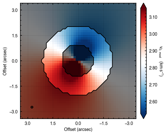
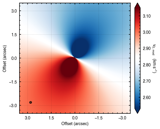
This can then be plotted through the plot_model convenience function.

[13]:

cube.plot_model(model=model)

../_images/tutorials_tutorial_1_43_0.png

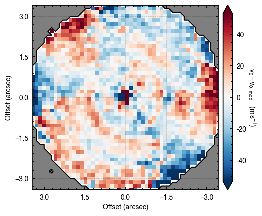
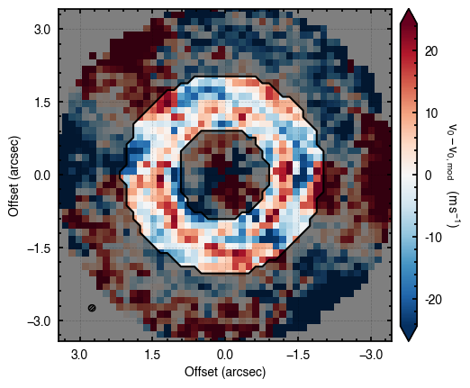
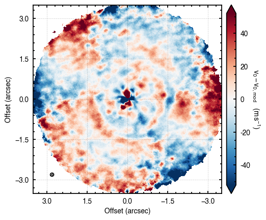
Similarly, we can plot the residuals with respect to the original data through plot_model_residuals.

[14]:

cube.plot_model_residual(model=model)

../_images/tutorials_tutorial_1_45_0.png

Both these functions can also directly take samples and params to skip the evaluate_models step.

However, this approach, which is used to make the plots generated with fit_map, is that it is assumed that the model parameters are independent such that taking the median of each posterior distribution provides the ‘best-fit’ model. Often parameteres are correlated and it is better to generate several realizations of the model from the posterior samples and then combine them. This can be achieved with the evaluate_models function and the draws argument.

[15]:

model = cube.evaluate_models(samples=samples, params=params, draws=100)
cube.plot_model(model=model)

../_images/tutorials_tutorial_1_47_0.png

Here the draws argument tells the function how many random draws to take which are then averaged down to a single value. If draws is less than 1, this represents the percentile of the posteriors to use (e.g., draws=0.5 will use the median values from all posterior distributions).

In addition, the evaluate_models function also allows for a user-defined function to collapse the multiple models, collapse_func. This is particularly useful if you want to see how much variability there is in the sample of models by looking at the standard deviation of the set. Note here how you can provide extra kwargs to the imshow function to display the data.

[16]:

scatter = cube.evaluate_models(samples=samples, params=params, draws=100, collapse_func=np.std)

fig, ax = plt.subplots()
im = ax.imshow(np.log10(scatter), origin='lower', extent=cube.extent, cmap='turbo', vmin=-0.5, vmax=1.0)
cb = plt.colorbar(im, extend='both')
cb.set_label(r'$\log_{10}\,\left(\delta v_0 \quad [{\rm m\,s^{-1}}] \right)$',
             rotation=270, labelpad=13)

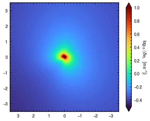
../_images/tutorials_tutorial_1_49_0.png

From this you can clearly see that there are small variations between the models in the posterior samples, but these are typically confined to the inner region of the disk.

Saving Models¶

If you want to save the model for use later, you can export it as a FITS cube, copying the header information from the attached FITS cube. As with evaluate_models, save_model accepts either the samples and params, or a pre-evaluated model.

[17]:

cube.save_model(model=model)

NOTE If the datacube has been clipped down using the FOV argument when loading the cube, the model will only populate pixels in that subregion. The rest will be left as NaN.